Calibration

Splitting data

For calibration and validation, we will use data from 2010 to 2015 and 2015 to 2020, respectively. The first year of each period will be dropped as a warm-up period. We first need to know how many days are in the calibration period.

get_num_days.py 2010-01-01 2015-12-31

Extract the first 2,191 records from input_evap.txt, input_pet.txt, and obs.txt.

head -9 input_evap.txt > input_c_evap.txt
tail +10 input_evap.txt | sed '2191q' >> input_c_evap.txt

head -9 input_pet.txt > input_c_pet.txt
tail +10 input_pet.txt | sed '2191q' >> input_c_pet.txt

head -2 obs.txt > obs_c.txt
tail +3 obs.txt | sed '2191q' >> obs_c.txt

We will use input_c_evap.txt, input_c_pet.txt, and obs_c.txt for calibration.

For validation, we will skip to January 1, 2015.

get_num_days.py 2010-01-01 2014-12-31

Skip the first 1,826 records from input_evap.txt, input_pet.txt, and obs.txt.

head -9 input_evap.txt > input_v_evap.txt
tail +1836 input_evap.txt >> input_v_evap.txt

head -9 input_pet.txt > input_v_pet.txt
tail +1836 input_pet.txt >> input_v_pet.txt

head -2 obs.txt > obs_v.txt
tail +1829 obs.txt >> obs_v.txt

We will use input_v_evap.txt, input_v_pet.txt, and obs_v.txt for validation.

Configuration

Open config.R.

nruns <- 1000
skip_c <- 365
skip_v <- 365
path_c <- list(params="params.txt",
           topidxstats="topidxstats.txt",
           input="input_c_pet.txt",
           output="output_c.txt",
           sim="sim",
           obs="obs_c.txt")
path_v <- list(params="params.txt",
           topidxstats="topidxstats.txt",
           input="input_v_pet.txt",
           output="output_v.txt",
           obs="obs_v.txt")

calc_nse <- function(obs, sim, skip=0){
    if(skip > 0){
            obs <- obs[-(1:skip)]
            sim <- sim[-(1:skip)]
    }
    1-sum((sim-obs)^2)/sum((mean(obs)-obs)^2)
}

calc_obj <- function(obs, sim, skip=0){
    1-calc_nse(obs, sim, skip)
}

nruns determines how many times to run r.topmodel for calibration. skip_c and skip_v are the numbers of time steps for warming up for calibration and validation, respectively. path_c and path_v define paths to input and output files for calibration and validation, respectively. Additionally, it defines a directory where simulation files for calibration will be saved (sim) and the location of an observed streamflow file (obs). calc_nse is the Nash-Sutclieffe efficiency (NSE) function. calc_obj is the objective function for minimization. Since this objective function returns 1 minus the NSE, its potential minimum value is 0, which means a perfect model.

Parametrization for ISPSO

Like many other optimization algorithms, ISPSO prefers normalized search spaces to reduce bias in certain parameter dimensions. The calibrate.R script takes parameter samples from a unit hypercube in \([0,1]^D\) where \(D\) is the number of dimensions or model parameters. This normalized search space is expanded to the r.topmodel parameter ranges linearly mapping 0 and 1 to the minimum and maximum parameter limits, respectively.

Running calibration

Create or empty the sim directory, copy params_init.txt to params.txt, and run calibrate.R. For this workshop, we use the Nash-Sutcliffe efficiency (NSE) coefficient as the objective function, but you can change it to another one in config.R.

cp params_init.txt params.txt
mkdir sim
# or rm sim/*

In R, install required packages and run calibrate.R.

install.packages(c("fOptions", "plotrix"))
source("../scripts/calibrate.R")

In a separate R session, inspect the declining pattern of the objective function.

repeat{
    obj <- read.table("sim/obj.txt")[[1]]; plot(cummin(obj), ylim=c(0, 0.5), type="l")
    cat(sprintf("obj=%f, NSE=%f\n", min(obj), 1-min(obj)))
    Sys.sleep(1)
}

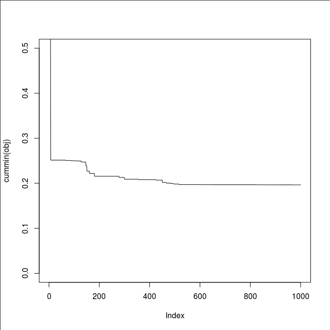
It took me about 2 minutes to populate the sim directory.

What is your best NSE 1-min(obj)? I got 0.8035311. Let’s validate this number.

source("config.R")
source("../scripts/run_rtopmodel.R")
source("../scripts/read_write_rtopmodel.R")

obj <- read.table("sim/obj.txt")[[1]]
x <- read.table("sim/x.txt")

best_idx <- which(obj==min(obj))
best_x <- as.numeric(x[best_idx,])

obs_c <- read.table("obs_c.txt")[[1]]
sim_c <- run_rtopmodel_x(best_x, path_c)
write.table(sim_c, "sim_c.txt", row.names=FALSE, col.names=FALSE)

calc_nse(obs_c, sim_c, skip_c)

This step will create the final output_c.txt and sim_c.txt.

Inspecting the calibration result

In R, let’s compare the observed and best simulated time series.

old.par <- par(mar=c(5.1, 4.5, 4.1, 2.1))
plot(obs_c[-(1:skip_c)], type="l", xlab="Time (days)", ylab=expression(Streamflow~(m^3/d)))
lines(sim_c[-(1:skip_c)], col="red")
legend("topleft", c("obs_c", "sim_c"), col=c("black", "red"), lty=c(1, 1), bty="n")

plot(obs_c, sim_c)
abline(0, 1, col="red")

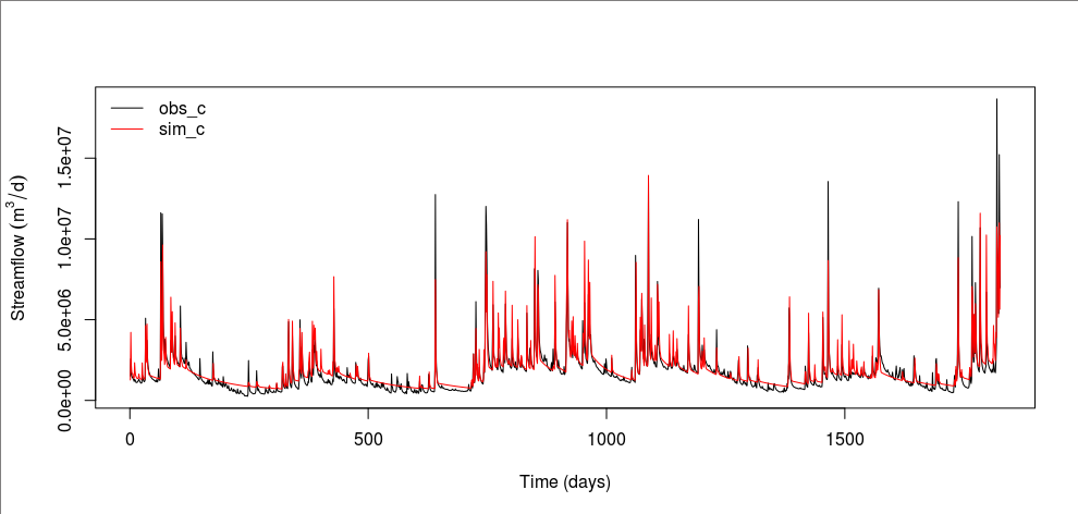
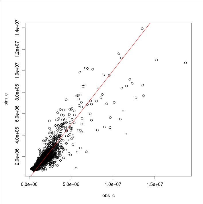
We can see that the best model tends to overestimate baseflows. Overall, simulated hydrographs decline at a slower rate than observed ones. This behavior might be attributed to the use of the NSE as the objective function because the NSE puts more weights on peak flows. It might be the single-watershed configuration or the infiltration calculation in r.topmodel. Probably, it might be the structure of TOPMODEL itself that has failed to simulate baseflows. Let’s see if r.topmodel has completely failed to simulate baseflows by plotting all 1,000 simulations. In the Generalized Likelihood Uncertainty Estimation (GLUE) framework (Beven and Binley, 2014), these simulations from the same model structure are called “models.”

sim_c <- c()
for(i in 1:1000){
    file <- sprintf("sim/sim_c_%04d.txt", i)
    sim_c <- rbind(sim_c, read.table(file)[[1]])
}

matplot(t(sim_c), type="l", col="green", lty=1)
lines(obs_c, col="red")
legend("topleft", legend=c("obs_c", "sim_c"), col=c("red", "green"), lty=1, bty="n")

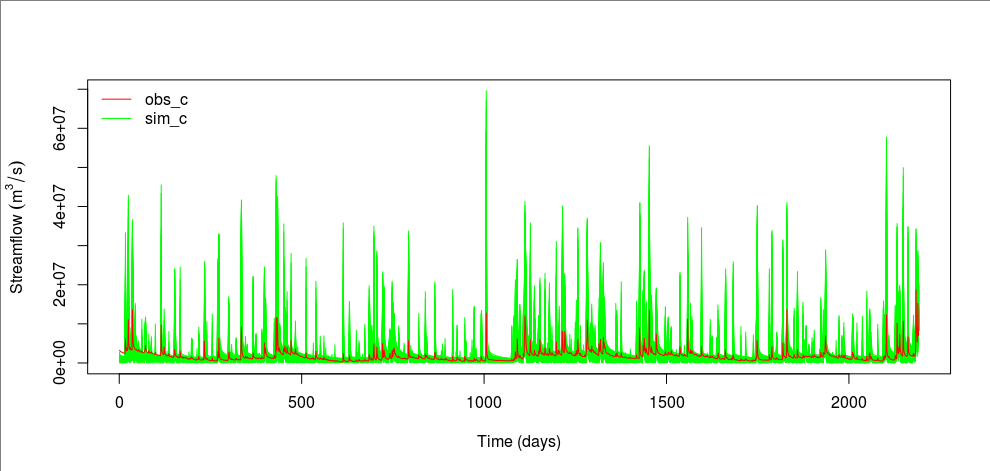
From the above plot, the observed streamflow is mostly within the simulated range. If we consider these “models” from the same model structure of TOPMODEL different models, constructing an ensemble model may be a good idea because no models are perfect and they all come with uncertainty.

References

Beven, K., Binley, A., 2014. GLUE - 20 Years On. Hydrological Processes 28 (24), 5897-5918. doi:10.1002/hyp.10082.