Random parameter sampling

Running r.topmodel with random parameter values

Without a priori knowledge about their distributions, we can assume that they follow a uniform distribution. If you want to take random parameter samples for Bayesian analysis under this assumption, you can use config_random.R and sample_random.R. This command will run r.topmodel 10,000 times and took about 20 minutes on my laptop, so you may just want to copy the sim_random directory to run/sim_random and skip to the next step for now.

mkdir sim_random
../scripts/sample_random.R

Performance comparison of calibration and random sampling

In R, let’s calculate the minimum objective function value.

obj_random <- read.table("sim_random/obj.txt")[[1]]
print(1-min(obj_random))

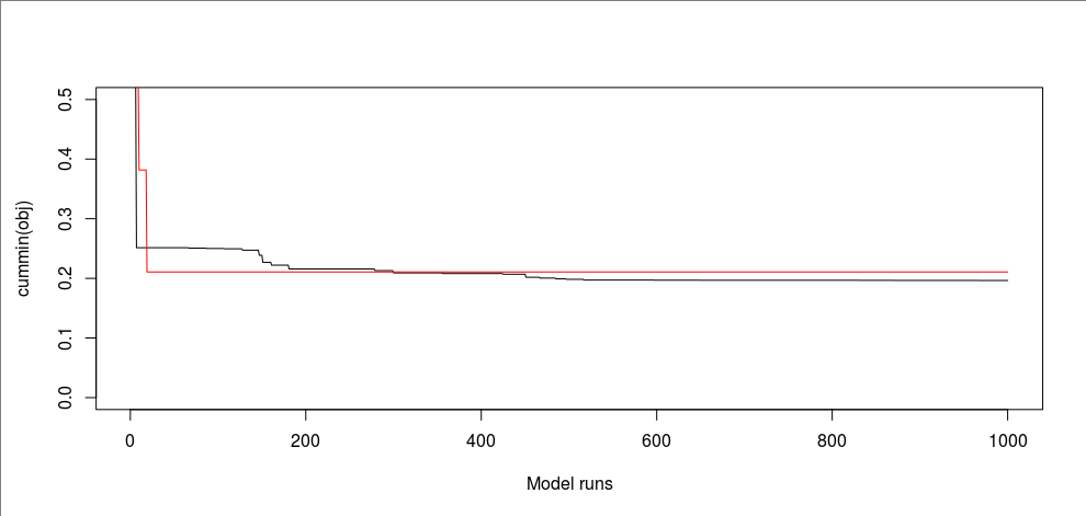
From this random sampling, I found an NSE of 0.7937873, which is slightly lower than 0.8035311 from our calibration. We can compare the performance of calibration and random sampling up to 1,000 runs if that matters.

obj <- read.table("sim/obj.txt")[[1]]

old.par <- par(mfrow=c(1,1), mar=c(5.1, 4.5, 4.1, 2.1))
plot(cummin(obj), ylim=c(0, 0.5), type="l", xlab="Model runs")
lines(cummin(obj_random[1:1000]), col="red")

This figure shows how fast calibration converges to the final state compared to random sampling.

Sensitivity analysis

Plot x-obj dotty plots to see how sensitive the objective function is to each parameter.

source("../scripts/run_rtopmodel.R")

x_random <- read.table("sim_random/x.txt")

old.par <- par(mfrow=c(2,5), mar=c(4.1, 4.1, 1.1, 1.1))
for(i in 1:10) plot(x_random[,i], obj_random, ylim=c(0,0.5), xlab=par.name[i], pch=20)

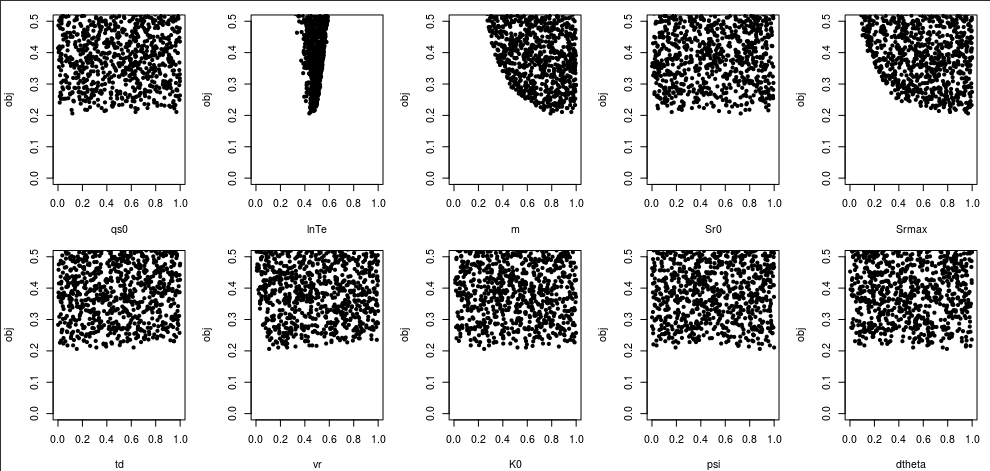
From these dotty plots, we can see that lnTe, m, and Srmax are sensitive parameters.

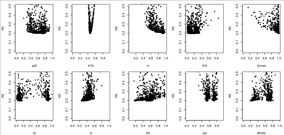
Let’s create a similar plot using the calibration result.

x <- read.table("sim/x.txt")
for(i in 1:10) plot(x[,i], obj, ylim=c(0,0.5), xlab=par.name[i], pch=20)